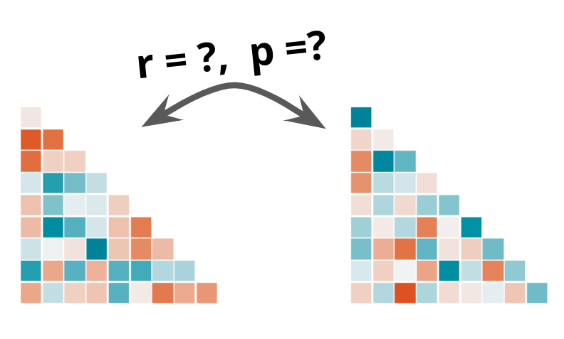
How to measure similarity between two correlation matrices
This post was also published in Towards Data Science on Medium
Tutorial on what metrics to use and how to calculate significance when measuring the similarity between matrices
Comparing the similarity between matrices can offer a way to assess the structural relationships among variables and is commonly used across disciplines such as neuroscience, epidemiology, and ecology.
Let’s assume you have data on how people react when watching a short Youtube video. This could be measured by facial expressions, heart rate, or breathing. A subject-by-subject similarity matrix of this data would represent how similar each person’s emotions were to every other subject. High similarity value in the matrix would mean that those individuals’ reactions were more similar than others.
You can compare this reaction similarity matrix with similarities in other factors such as demographics, interests, and/or preferences. This allows you to directly test if similarities in one domain (e.g. emotional reactions) can be explained by similarities in another (e.g. demographic/preference similarities).
This tutorial introduces the different metrics that can be used to measure similarity between similarity matrices and how to calculate the significance of those values.
Step 0: Preparing the data
Let’s simulate some data for analysis. We create a random data m1_u and m2_u that are related by the amount of noise added nr. Next, we create a correlation matrix for each underlying data using the default pandas correlation function. Let’s assume that the correlation matrix m1 represents how similar each subject’s reactions were to every other subject and m2 represents how similar each subject’s preferences were to one another. We can simulate and visualize these matrices with the following code.
import seaborn as sns
import numpy as np
import pandas as pd
import scipy.stats as stats
from scipy.spatial.distance import squareform
import matplotlib.pyplot as plt

# n is the number of subjects or items that will determine the size of the correlation matrix.
n = 20
data_length = 50
nr = .58

# Random data
np.random.seed(0)
m1_u = np.random.normal(loc=0, scale=1, size=(data_length, n))
m2_u = nr*np.random.normal(loc=0, scale=1, size=(data_length, n)) + (1-nr)*m1_u

m1 = pd.DataFrame(m1_u).corr()
m2 = pd.DataFrame(m2_u).corr()

f,axes = plt.subplots(1,2, figsize=(10,5))
sns.set_style("white")
for ix, m in enumerate([m1,m2]):
  sns.heatmap(m, cmap="RdBu_r", center=0, vmin=-1, vmax=1, ax=axes[ix], square=True, cbar_kws={"shrink": .5}, xticklabels=True)
  axes[ix].set(title=f"m{ix+1}")
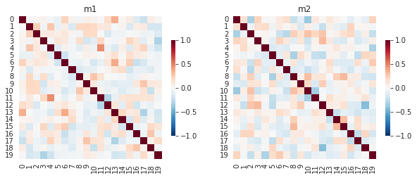
Correlation matrices m1 and m2.
Now let’s see how we can test the similarity of these two matrices.
Step 1: Measuring the similarity between two correlation matrices.
To measure the similarity between two correlation matrices you first need to extract either the top or the bottom triangle. They are symmetric but I recommend extracting the top triangle as it offers more consistency with other matrix functions when recasting the upper triangle back into a matrix.
The way to extract the upper triangle is simple. You can use the following function upper which leverages numpy functionality triu_indices. We can see from the figure below that the extracted upper triangle matches the original matrix.
def upper(df):
    '''Returns the upper triangle of a correlation matrix.
    You can use scipy.spatial.distance.squareform to recreate matrix from upper triangle.
    Args:
      df: pandas or numpy correlation matrix
    Returns:
      list of values from upper triangle
    '''
    try:
        assert(type(df)==np.ndarray)
    except:
        if type(df)==pd.DataFrame:
            df = df.values
        else:
            raise TypeError('Must be np.ndarray or pd.DataFrame')
    mask = np.triu_indices(df.shape[0], k=1)
    return df[mask]

# Compare that the upper triangle is properly extracted.
print("Extracted upper triangle from m1")
print(np.round(upper(m1)[:25],3))
print("Top 3 rows from m1")
display(m1.iloc[:3, :].round(3))
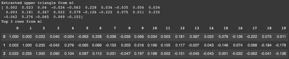
Figure comparing the extracted values from the upper matrix to the actual top portion of the matrix.
Now that you have the matrices in simple vector forms, you can use the metric you need to measure similarity. The precise metric you use will depend on the properties of data you are working with but it is recommended to use a rank correlation such as a Spearman’s ρ or a Kendall’s τ. The benefit is that you don’t need to assume that similarity increases are linear and results will also be more robust to outliers.
In this example, let’s use the Spearman correlation to measure the similarity.
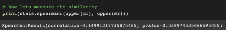
# Now lets measure the similarity
print(stats.spearmanr(upper(m1), upper(m2)))
Which yields the following result of a Spearman rho of .15. The Spearman function also offers a p-value of .038, but using this would be inaccurate. Our data is non-independent meaning that each cell value from the upper matrix cannot be taken out independently without affecting other cells that arise from the same subject (learn more here). Alternatively, we can use the permutation testing approach outlined in Step 2.
Spearman rank correlation between correlation matrices m1 and m2. Figure produced by author.
Step 2: Testing significance with permutations.
Each cell value from our upper matrices are non-independent from one another. The independence is at the level of the subject which will be what we would be permuting.
In each iteration of the for loop in the function below, we shuffle the order of rows and columns from one of the correlation matrices, m1. We re-calculate the similarity between two matrices the amount of time we want to permute (e.g. 5000 times). After that, we can see how many values fall above our estimated value to obtain a p-value.
"""Nonparametric permutation testing Monte Carlo"""
np.random.seed(0)
rhos = []
n_iter = 5000
true_rho, _ = stats.spearmanr(upper(m1), upper(m2))
# matrix permutation, shuffle the groups
m_ids = list(m1.columns)
m2_v = upper(m2)
for iter in range(n_iter):
  np.random.shuffle(m_ids) # shuffle list
  r, _ = stats.spearmanr(upper(m1.loc[m_ids, m_ids]), m2_v)
  rhos.append(r)
perm_p = ((np.sum(np.abs(true_rho) <= np.abs(rhos)))+1)/(n_iter+1) # two-tailed test


f,ax = plt.subplots()
plt.hist(rhos,bins=20)
ax.axvline(true_rho,  color = 'r', linestyle='--')
ax.set(title=f"Permuted p: {perm_p:.3f}", ylabel="counts", xlabel="rho")
plt.show()
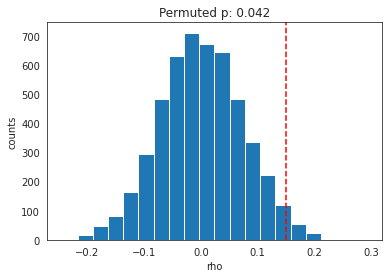
Permutation results. Red dotted line indicates true rho.
As shown in the figure above, our permuted p is more conservative at p=.042 than the one we obtained earlier at p=.038.
Final thoughts
Comparing similarity matrices can help identify shared latent structures in the data across modalities. This tutorial offers a basic approach to assessing the similarity and calculating significance with a non-parametric permutation testing.
This approach can be extended in many ways. One extension would be to compare the average level of similarity between two correlation matrices. You can use the same approach of extracting the upper triangle and permuting the data to get significance for the difference. One thing to add however is that you’ll want to convert the Pearson’s R into a Z distribution using the Fisher transformation to make the distribution approximately normal.
Another extension would be to compare two distance matrices, such as geographical distance, Euclidean distance, or Mahalanobis distance. All you have to do is to create a distance matrix rather than correlation matrix. A real-world example with data comparing how distance between cities relates to average temperature differences is included in the full Colab notebook in the link below.
Here is a Google Colab Jupyter Notebook to run all the tutorials.
machine-learning statistics data-science python