Three ways to run Linear Mixed Effects Models in Python Jupyter Notebooks

Photo by Forest Simon on Unsplash
This post was also published in Towards Data Science on Medium
Tutorial on how to run Linear Mixed Effects Regressions (LMER) models in Python and Jupyter Notebooks
One of the reasons I could not fully switch out of R to Python for data analyses was that linear mixed effects models used to be only available in R. Linear mixed effects models are a strong statistical method that is useful when you are dealing with longitudinal, hierarchical, or clustered data. Simply put, if you have repeated samples or correlated data due to natural “groupings” in such as repeated responses from the same individuals over time, repeated data from different geographical locations, or even data from a group interaction experiment, you would probably want to use linear mixed effects models for your analyses.
You can learn more about exactly how linear mixed effects models or linear mixed effects regressions (LMER) are useful in these resources: (Lindstrom & Bates, 1988) (Bates et al., 2015). This tutorial, will focus on how you can run these analyses in a Python environment. In the early days, I had save the data from Python open up the data in R and run the model. Over the years, things became more convenient and several convenient options have emerged. Here are three options for which I provide a quick tutorial:
- LMER in Statsmodels
- Accessing LMER in R using rpy2 and %Rmagic
- Pymer4 for seamless access to LMER in R
Here is a Google Colab Jupyter Notebook to follow along these methods.
LMER in Statsmodels
Currently, the simples solutions is to use the LMER implementation in the Statsmodels package, with examples here. Installation is simple as pip install statsmodels. After installation, you can run LMER with the following.
!pip install -q statsmodels
import numpy as np
import pandas as pd
import statsmodels.api as sm
import statsmodels.formula.api as smf
data = sm.datasets.get_rdataset('dietox', 'geepack').data
md = smf.mixedlm("Weight ~ Time", data, groups=data["Pig"], re_formula="~Time")
mdf = md.fit(method=["lbfgs"])
print(mdf.summary())
To provide a bit more context, we are analyzing the dietoxdataset (learn more about the dataset here) to predict the weight of pigs as a function of time with a random slope specified by re_formula=”~Time” and a random intercept automatically specified by groups=data[“Pig”]. The outputs look like the figure below with the coefficients, standard errors, z stats, p values, and 95% confidence intervals.
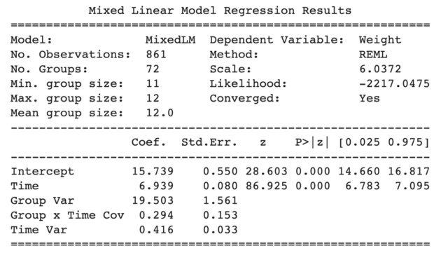
Statsmodels LMER outputs
While this is splendid, specifying the random effects is somewhat inconvenient and diverges from the formulaic expressions used in LMER in R. For example in R, the random slopes and intercepts are specified within the model formula in one line, such as:
lmer('Weight ~ Time + (1+Time|Pig)', data=dietox)
This leads to our second option of using LMER in R through a direct interface between Python and R through Rpy2.
Accessing LMER in R using rpy2 and %Rmagic
The second option is to directly access the original LMER packages in R through the rpy2 interface. The rpy2 interface allows users to toss data and results back and forth between your Python Jupyter Notebook environment and your R environment. rpy2 used to be notoriously finicky to install, but it has gotten more stable over the years. To use this option, you’ll need to install R in your machine as well as rpy2 which can be achieved in Google Colab with the following code:
!apt-get install r-base
!pip install -q rpy2
packnames = ('lme4', 'lmerTest', 'emmeans', "geepack")
from rpy2.robjects.packages import importr
from rpy2.robjects.vectors import StrVector
utils = importr("utils")
utils.chooseCRANmirror(ind=1)
utils.install_packages(StrVector(packnames))
The first line installs R using Linux syntax. If you are using a Mac or Windows you can achieve this by simply following the R installation instructions. The next set of lines install rpy2 then uses rpy2 to install the lme4 andlmerTest packages. Next, you’ll need to activate the Rmagic through the code
%load_ext rpy2.ipython
After this, by starting your Jupyter Notebook cell with %%R will allow you to run R command from your notebook. For example, to run the same model that we ran in statsmodels, you would run the following:
# make sure rpy2 was loaded using %load_ext rpy2.ipython
%%R
library(lme4)
library(lmerTest)
data(dietox, package='geepack')
m<-lmer('Weight ~ Time + (1+Time|Pig)', data=dietox)
print(summary(m))
Note that this code starts with %%R which signals that this cell contains R code. We are also using a much simpler formulaic expression than statsmodels, We were able to specify that our groupings is Pigs and that we are estimating both random slopes and intercepts through (1+Time|Pig). This will give you the results that you would be more familiar with if you had been using LMER in R.
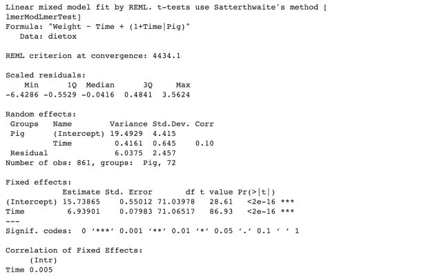
LMER output from rpy2
And as I mentioned earlier, you can also pass your Pandas DataFrames to R. Remember that data DataFrame we loaded earlier? We can pass that to R, run the same LMER model, and retrieve the coefficients like this.
%%R -i data -o betas
m<-lmer('Weight ~ Time + (1+Time|Pig)', data=data)
print(summary(m))
betas <- fixef(m)
The -i data sends our Python Pandas DataFramedata into R and we use that to estimate our model m. Next, we retrieve the betas coefficients from the model with beta <- fixef(m) which is exported back to our notebook, because we specified in the first line -o betas.
The best part of this approach is that you can add additional code in the R environment before running the model. For example, maybe you want to make sure a column called Evit is recognized as a factor with data$Evit <- as.factor(data$Evit), specify a new contrast for this categorical variable using contrasts(data$Evit) <- contr.poly , or even relevel your categorical data in the formula itself. All this can be easily achieved when using rpy2 to access LMER from R.
%%R -i data
# Specify Evit as a factor and set a polynomial contrast.
data$Evit <- as.factor(data$Evit)
contrasts(data$Evit) <- contr.poly
m<-lmer('Weight ~ Time * Evit + (1|Pig)', data=data)
print(summary(m))

# Relevel categorical data so base level is Evit100
m<-lmer('Weight ~ Time * relevel(Evit, ref="Evit100") + (1|Pig)', data=data)
print(summary(m))
To summarize, rpy2 interface gives you the most flexibility and the ability to access LMER and additional functions in R which you might be more familiar with if you are transitioning from R to Python. Lastly, we’ll touch a middle ground option using the Pymer4 package.
LMER with Pymer4
Pymer4 (Jolly, 2018) can be a convenient middle ground between using LMER directly through rpy2 and using an LMER implementation in Statsmodels. This package basically brings you the convenience of using R formulaic syntax but in a more Pythonic way, without having to deal with the R magic cells.
# Install pymer4
!pip install -q pymer4
# load pymer4
from pymer4.models import Lmer
model = Lmer('Weight ~ Time + Evit + (1 + Time|Pig)', data=data)
display(model.fit())
# ANOVA results from fitted model
display(model.anova())
# Plot estimated model coefficients
model.plot_summary()
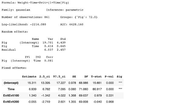
LMER output from Pymer4
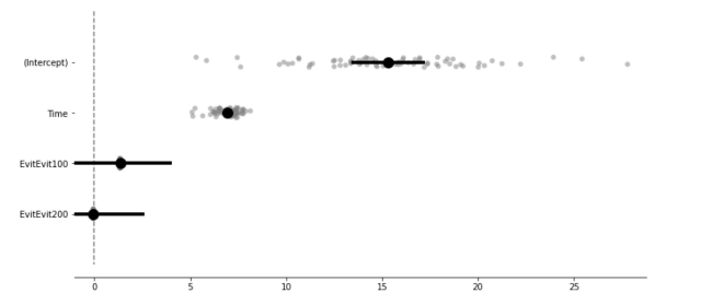
Estimated values including random intercept and slope estimates.
Conclusion
We covered 3 ways to run Linear Mixed Effects Models from a Python Jupyter Notebook environment. Statsmodels can be the most convenient but the syntax might be unfamiliar to users already experienced with LMER in R syntax. Using rpy2 gives you the most flexibility and power but this can get messy as you need to use Rmagic to switch between Python and R cells. Pymer4 is the great compromise solution which provides convenient access to LMER in R while minimizing the switch cost between languages. \
Here is a Google Colab Jupyter Notebook to run all the tutorials.
machine-learning statistics data-science python r