This notebook is designed to serve as an introduction to signal processing and synchrony measures between timeseries using instantaneous phase synchrony and rolling window correlations.

Content

Signal processing with Fourier Transform
Instantaneous Phase Synchrony between two timeseries
Rolling Window Correlation Synchrony between two timeseries
Comparison between Instantaneous Phase Synchrony and Window Correlations Synchrony

# Load basic functions
from scipy.signal import hilbert, butter, filtfilt
from scipy.fftpack import fft,fftfreq,rfft,irfft,ifft
import numpy as np
import seaborn as sns
import pandas as pd
import scipy.stats as stats
%matplotlib inline
import matplotlib.pyplot as plt
import matplotlib as mpl
sns.set_context('poster',font_scale=.8)
sns.set_style('whitegrid')
mpl.rc('figure',figsize=(15,2))

1. Signal processing with Fourier Transform

Fourier transform decomposes a timeseries data into a combination of signals at different frequencies. It allows you to analyze timeseries data at the frequency level to determine what frequency bands of your signal is noise and what frequency band is actual data.

The other nice characteristic of the Fourier is that it provides a one-to-one mapping with the original signal so that you can go back and forth between the original and transformed signal. Once can even filter out different frequency bands using this method (although the preferred way would be to use a bandpass filter).

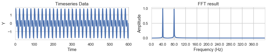
First lets generate a sample timeseries y1 which will be combination of sin waves with frequencies 40Hz and 80Hz. We plot the wave data on the left, and the FFT transformed data on the right.
The FFT result on the right show that we succesfully determined that our data is composed of a 40Hz signal and a 80Hz signal.

# Simulate Timeseries Data
N = 600 # number of smaples
T = 1.0 / 800.0 # sample spacing
x = np.linspace(0.0, N*T, N) # generate x
y1 = np.sin(40.0 * 2.0*np.pi*x)+np.sin(80.0 * 2.0*np.pi*x) # generate data

f,ax=plt.subplots(1,2,figsize=(15,2))
# plot timeseries
ax[0].plot(y1)
ax[0].set(ylabel='Y',xlabel='Time',title='Timeseries Data',xlim=[0,N])
# Plot fft
ticksteps = 30
yf = fft(y1) # perform FFT
amp = 2.0/N * np.abs(yf)
ax[1].plot(amp[:N//2])
ax[1].set(xticks=(np.arange(0,N//2,ticksteps)), ylabel='Amplitude',xlabel='Frequency (Hz)',title='FFT result',xlim=[0,N//2])
ax[1].set_xticklabels(np.round(fftfreq(N,T)[:N//2],2)[::ticksteps],rotation=0)
plt.show()

png

2. Instantaneous phase synchrony between two timeseries.

The instantaneous phase synchrony measures the phase similarities between signals at each timepoint.
The phase refers to the angle of the signal when it is resonating between 0 ~ 360 degrees or -pi to pi degrees. When two signals line up in phase their angular difference becomes zero. The angles can be calculated through the hilbert transform of the signal. Phase coherence can be quantified by subtracting the angular difference from 1.

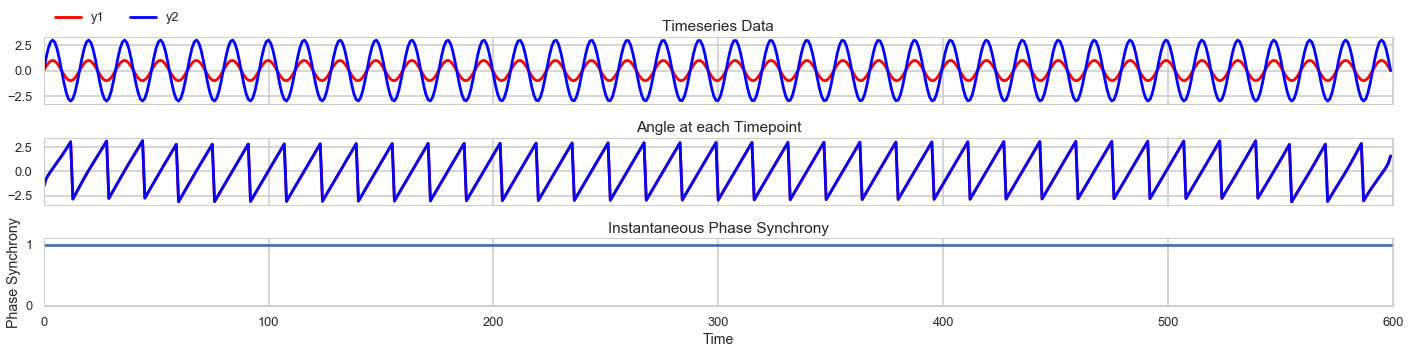
First we simulate a signal with perfect phase synchrony. Both signals y1 and y2 are at 50Hz.
The angles of the signal are perfectly in sync, so they instantaneous coherence measure is always at 1.

N = 600 # number of smaples
T = 1.0 / 800.0 # sample spacing
x = np.linspace(0.0, N*T, N)
phase_y1, phase_y2 = 50., 50.
amp_y1, amp_y2 = 1.,3.
y1 = amp_y1*np.sin(phase_y1 * 2.0*np.pi*x)
y2 = amp_y2*np.sin(phase_y2 * 2.0*np.pi*x)
window=10
al1 = np.angle(hilbert(y1),deg=False)
al2 = np.angle(hilbert(y2),deg=False)
f,ax = plt.subplots(3,1,figsize=(20,5),sharex=True)
ax[0].plot(y1,color='r',label='y1')
ax[0].plot(y2,color='b',label='y2')
ax[0].legend(bbox_to_anchor=(0., 1.02, 1., .102),ncol=2)
ax[0].set(xlim=[0,N], title='Timeseries Data')
ax[1].plot(al1,color='r')
ax[1].plot(al2,color='b')
ax[1].set(title='Angle at each Timepoint')
phase_synchrony = 1-np.sin(np.abs(al1-al2)/2)
ax[2].plot(phase_synchrony)
ax[2].set(ylim=[0,1.1],xlim=[0,N],title='Instantaneous Phase Synchrony',xlabel='Time',ylabel='Phase Synchrony')
plt.tight_layout()
plt.show()

png

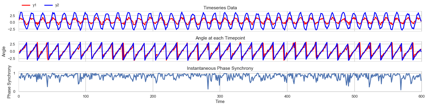
We can also add random noise to the data and see how it changes the results.
The fluctuating phase synchrony graph indiates that instantaneous phase synchrony can be sensitive to noise
and highlights the importance of filtering and choosing a frequency band for analysis.

N = 600 # number of smaples
T = 1.0 / 800.0 # sample spacing
x = np.linspace(0.0, N*T, N)
phase_y1, phase_y2 = 50., 50.
amp_y1, amp_y2 = 1.,3.
y1 = amp_y1*np.sin(phase_y1 * 2.0*np.pi*x)+np.random.rand(N)
y2 = amp_y2*np.sin(phase_y2 * 2.0*np.pi*x)+np.random.rand(N)
window=10
al1 = np.angle(hilbert(y1),deg=False)
al2 = np.angle(hilbert(y2),deg=False)
f,ax = plt.subplots(3,1,figsize=(20,5),sharex=True)
ax[0].plot(y1,color='r',label='y1')
ax[0].plot(y2,color='b',label='y2')
ax[0].legend(bbox_to_anchor=(0., 1.02, 1., .102),ncol=2)
ax[0].set(xlim=[0,N], title='Timeseries Data')
ax[1].plot(al1,color='r')
ax[1].plot(al2,color='b')
ax[1].set(ylabel='Angle',title='Angle at each Timepoint')
phase_synchrony = 1-np.sin(np.abs(al1-al2)/2)
ax[2].plot(phase_synchrony)
ax[2].set(ylim=[0,1.1],xlim=[0,N],title='Instantaneous Phase Synchrony',xlabel='Time',ylabel='Phase Synchrony')
plt.tight_layout()
plt.show()

png

3. Rolling Window Correlation Synchrony between two timeseries

Windowed correlations are widely used because of their simplicity.
When filtering is difficult due to missing data or uncertainty about which frequencies to analyze, windowed correlation can be a good approximation of synchrony between two signals.

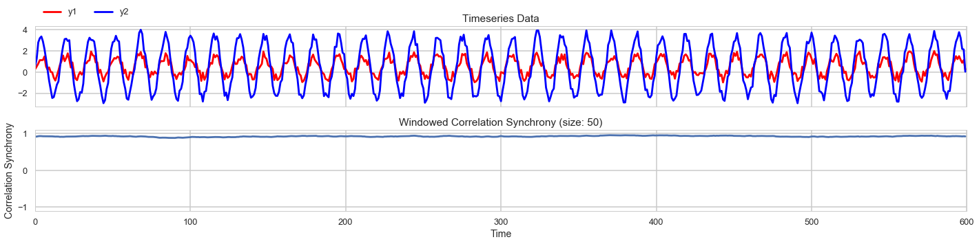
We look at the window correlation of two timeseries both at 50Hz and with added random noise.
The correlation synchrony results indicate that the window correlation measure provides a much more stable measure of synchrony robust to the high frequency random noise.

For the window correlation I use a customized function that utilizes the Pandas rolling function but that pads each end of data so that it provides values for each ends as well.

def get_triangle(df,k=0):
    '''
    This function grabs the upper triangle of a correlation matrix
    by masking out the bottom triangle (tril) and returns the values.

    df: pandas correlation matrix
    '''
    x = np.hstack(df.mask(np.tril(np.ones(df.shape),k=k).astype(np.bool)).values.tolist())
    x = x[~np.isnan(x)]
    return x  

def rolling_correlation(data, wrap=False, *args, **kwargs):
    '''
    Intersubject rolling correlation.
    Data is dataframe with observations in rows, subjects in columns.
    Calculates pairwise rolling correlation at each time.
    Grabs the upper triangle, at each timepoints returns dataframe with
    observation in rows and pairs of subjects in columns.
    *args:
        window: window size of rolling corr in samples
        center: whether to center result (Default: False, so correlation values are listed on the right.)
    '''
    data_len = data.shape[0]
    half_data_len = int(data.shape[0]/2)
    start_len = data.iloc[half_data_len:].shape[0]
    if wrap:
        data = pd.concat([data.iloc[half_data_len:],data,data.iloc[:half_data_len]],axis=0).reset_index(drop=True)
    _rolling = data.rolling(*args, **kwargs).corr()       
    rs=[]
    for i in np.arange(0,data.shape[0]):
        rs.append(get_triangle(_rolling.loc[i]))
    rs = pd.DataFrame(rs)   
    rs = rs.iloc[start_len:start_len+data_len].reset_index(drop=True)
    return rs  

N = 600 # number of smaples
T = 1.0 / 800.0 # sample spacing
x = np.linspace(0.0, N*T, N)
window_size = 50
phase_y1, phase_y2 = 50., 50.
amp_y1, amp_y2 = 1.,3.
y1 = amp_y1*np.sin(phase_y1 * 2.0*np.pi*x)+np.random.rand(N)
y2 = amp_y2*np.sin(phase_y2 * 2.0*np.pi*x)+np.random.rand(N)
window=10
al1 = np.angle(hilbert(y1),deg=False)
al2 = np.angle(hilbert(y2),deg=False)
f,ax = plt.subplots(2,1,figsize=(20,5),sharex=True)
ax[0].plot(y1,color='r',label='y1')
ax[0].plot(y2,color='b',label='y2')
ax[0].legend(bbox_to_anchor=(0., 1.02, 1., .102),ncol=2)
ax[0].set(xlim=[0,N], title='Timeseries Data')
window_corr_synchrony = rolling_correlation(data=pd.DataFrame({'y1':y1,'y2':y2}),wrap=True,window=window_size,center=True)
window_corr_synchrony.plot(ax=ax[1],legend=False)
ax[1].set(ylim=[-1.1,1.1],xlim=[0,N],title='Windowed Correlation Synchrony (size: '+str(window_size)+')',xlabel='Time',ylabel='Correlation Synchrony')
plt.tight_layout()
plt.show()

png

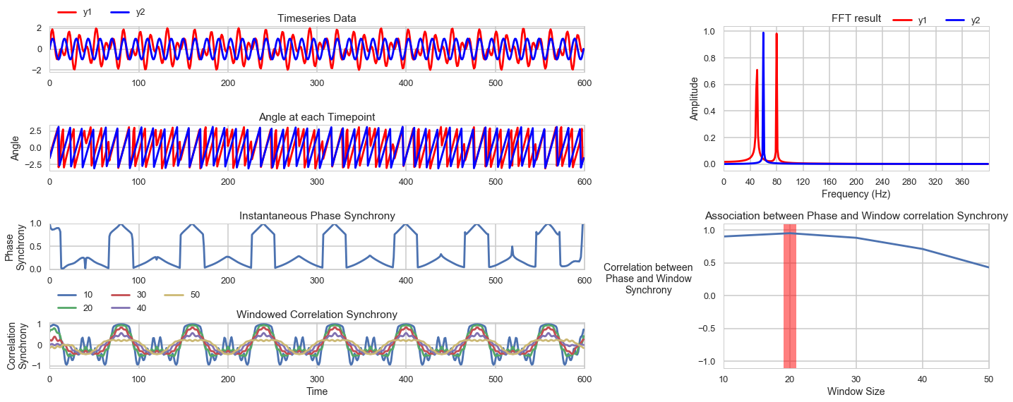
4. Comparison between Instantaneous Phase Synchrony and Windowed Correlations Synchrony

Mangor Pedersen at Florey Institute of Neuroscience has a preprint on the relationship between the instantaneous phase synchrony and windowed correlations for fMRI data. The gist of it is that the two are highly correlated with the correct window. Different window sizes are compared with data bandpass filtered at 0.03~0.07 Hz and 0.01-0.1 Hz with the results showing that a window length of 19~20 seconds provides highest similarity between phase synchrony and windowed synchrony measures. It is intriguing that this is the approximate length of the hemodynamic function and that both frequency bands include the 20 second signal 0.01Hz (100 seconds) ~ 0.1Hz (10 seconds).

Here is a simulation comparing the phase synchrony and windowed correlation measures. Not sure if there is a clear mathematical relationship between the two, in that we could derive the optimal window based on the signal. Nevertheless, it seems that careful selection of the window size can provide a connection between the two synchrony measures.

N = 600 # number of smaples
T = 1.0 / 800.0 # sample spacing
x = np.linspace(0.0, N*T, N)
window_sizes = [10,20,30,40,50]
window_sizes = np.arange(10,51,10).astype(int)
phase_y1_1,phase_y1_2, phase_y2 = 80., 50., 60
amp_y1, amp_y2 = 1., 1.
y1 = amp_y1*np.sin(phase_y1_1 * 2.0*np.pi*x) + amp_y1*np.sin(phase_y1_2 * 2.0*np.pi*x)
y2 = amp_y2*np.sin(phase_y2 * 2.0*np.pi*x)
al1 = np.angle(hilbert(y1),deg=False)
al2 = np.angle(hilbert(y2),deg=False)
f = plt.figure(figsize=(20,8))
gs = mpl.gridspec.GridSpec(4,8)
ax=[f.add_subplot(gs[0,:5]), f.add_subplot(gs[1,:5]),
    f.add_subplot(gs[2,:5]),f.add_subplot(gs[3,:5]),
    f.add_subplot(gs[:2,5:]), f.add_subplot(gs[2:,5:])]
ax[0].plot(y1,color='r',label='y1')
ax[0].plot(y2,color='b',label='y2')
ax[0].legend(bbox_to_anchor=(0., 1.02, 1., .102),ncol=2)
ax[0].set(xlim=[0,N], title='Timeseries Data')
ax[1].plot(al1,color='r')
ax[1].plot(al2,color='b')
ax[1].set(ylabel='Angle', xlim=[0,N],title='Angle at each Timepoint')
phase_synchrony = 1-np.sin(np.abs(al1-al2)/2)
ax[2].plot(phase_synchrony)
ax[2].set(ylim=[0,1],xlim=[0,N],title='Instantaneous Phase Synchrony',ylabel='Phase\nSynchrony')
window_corr_synchrony = pd.DataFrame(columns=window_sizes,index=np.arange(0,N))
for window_size in window_sizes:
    window_corr_synchrony[window_size]=rolling_correlation(data=pd.DataFrame({'y1':y1,'y2':y2}),wrap=True,window=window_size,center=True)
window_corr_synchrony.plot(ax=ax[3])
ax[3].legend(bbox_to_anchor=(0., 1.02, 1., .102),ncol=3)
ax[3].set(ylim=[-1.1,1.1],xlim=[0,N],title='Windowed Correlation Synchrony',xlabel='Time',ylabel='Correlation\nSynchrony')

ticksteps = 30
yf1,yf2 = fft(y1),fft(y2) # perform FFT
amp1,amp2 = 2.0/N * np.abs(yf1),2.0/N * np.abs(yf2)
ax[4].plot(amp1[:N//2],color='r',label='y1')
ax[4].plot(amp2[:N//2],color='b',label='y2')
ax[4].set(xticks=(np.arange(0,N//2,ticksteps)), ylabel='Amplitude',xlabel='Frequency (Hz)',title='FFT result',xlim=[0,N//2])
ax[4].set_xticklabels([int(_tick) for _tick in np.round(fftfreq(N,T)[:N//2],2)[::ticksteps]],rotation=0)
ax[4].legend(bbox_to_anchor=(0., 1.02, 1., .102),ncol=3)

rs_per_window = pd.DataFrame(columns=['rs'],index=np.arange(min(window_sizes),max(window_sizes)+1,1))
rs_per_window['rs']=np.nan
for window_size in window_sizes:
    rs_per_window.loc[window_size,'rs'] = (np.round(stats.pearsonr(phase_synchrony,window_corr_synchrony[window_size].values.ravel())[0],2))
rs_per_window.interpolate(method='index').plot(ax=ax[5],legend=False)
ax[5].set(xticks=window_sizes,xticklabels=[int(w) for w in window_sizes],ylim=[-1.1,1.1],xlabel='Window Size',title='Association between Phase and Window correlation Synchrony')
ax[5].set_ylabel('Correlation between\nPhase and Window\nSynchrony',rotation=0,labelpad=70)
rs_bool = rs_per_window==rs_per_window.max()
rs_bool.loc[rs_per_window.idxmax().values[0]-1:rs_per_window.idxmax().values[0]+1]=True
ax[5].fill_between(np.arange(min(window_sizes),max(window_sizes)+1,1),-1.1,1.1,where=rs_bool.values.ravel(),facecolor='red',alpha=.5)
plt.tight_layout()
plt.show()

png

Conclusion

If the signal to be analyzed has a well-defined frequency range, instantaneous phase synchrony relieves the burden of having to subjectively define a window size. However, if the signal is not well filtered due to missing data or the frequency band is large, a rolling window correlation can also provide a robust measure of synchrony.